What is a directed acyclic graph (DAG)?

Caroline Morton

November 12, 2026
In my previous post on confounders, I discussed an example where birth order appeared to influence the risk of Down syndrome. Babies born later in a family seemed to have a higher risk, and the important factor was found to be maternal age, which is associated with both birth order and the likelihood of having a baby with Down syndrome. This is a good example of why we need to think carefully about the relationships between variables, as just because two things are associated, doesn’t necessarily mean that one causes the other.
One way epidemiologists make sense of relationships between variables is visualising them using directed acyclic graphs, or DAGs. A DAG is a diagram that represents our assumptions about how different variables cause or influence one another. It’s also particularly useful for identifying which variables we should adjust for in a statistical analysis and which we shouldn’t. The name itself is also descriptive, where directed means the arrows have a direction, acyclic means you can’t follow the arrows in a loop back to the starting point, and graph refers to the diagram.
In this post, I’ll explain how DAGs work using a couple of examples. For a more technical explanation, I’d recommend Digitale and colleagues’ tutorial on DAGs, which also provides some useful examples of how they are applied in epidemiological research.
How do we read a DAG?
Let’s take a deeper look at the birth-order example and map out the relationships between the three variables.
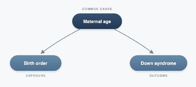
The diagram shows maternal age on top, with two arrows pointing towards birth order and Down syndrome. Each of the three variables is represented as a node, and the arrows show the direction of the assumed causal relationships. Maternal age influences birth order because women are older when having their second or third children. Meanwhile, age also influences the risk of having a baby with Down syndrome. As you can see on the DAG, there is no arrow between birth order and Down syndrome, because we’re assuming that birth order itself doesn’t cause Down syndrome.
This is a really important point about DAGs. While every arrow represents an assumption about cause and effect, leaving an arrow out is also in itself an assumption. No arrow means we’re assuming there is no direct causal effect between those variables, and we made this assumption, based on what we already know or believe about how the world works, drawing on our own previous research and subject knowledge.
How do DAGs distinguish causal from non-causal relationships?
One important thing to notice about the birth order example is that two variables can be associated without one causing the other, and a DAG can help us understand which are causal and non-causal paths by looking at the direction of the arrows.
- A causal path follows arrows forwards, from a cause towards an outcome. For example, if smoking causes lung cancer, the arrow would point from smoking towards lung cancer.
- A non-causal path connects two variables on the diagram, but the arrows don’t all point forwards from the exposure to the outcome, so the path doesn’t represent a causal effect.
If you take another look at the birth order DAG, you can see there is a non-causal path connecting birth order with Down syndrome through maternal age. Maternal age influences both variables, which means that birth order and Down syndrome can appear associated, even though birth order itself doesn’t cause Down syndrome. This is what we call confounding, and the route through maternal age is known as a backdoor path.
One way we can account for this confounding is to adjust for maternal age. For example, instead of comparing first-born babies with later-born babies, we can compare babies born to mothers of the same age. Because maternal age is the same across both comparison groups, it can’t be the cause of the difference in Down syndrome risk.
How can adjusting for a variable cause problems?
While adjusting for a confounder can help us mitigate its effects on the results, adjusting for, or selecting participants based on other variables can sometimes introduce bias into the analysis. One example of this is described in a hypothetical study by Digitale and colleagues, investigating the relationship between the number of sexual partners and cervical cancer.
They described a scenario where participants were recruited through a sexual health clinic. Suppose people with more sexual partners are more likely to attend the clinic because of an increased risk of sexually transmitted infections (STIs), while people with cervical cancer could be attending because some of the early symptoms can be mistaken for an STI. This is shown in the DAG below, where you can see both the exposure (number of sexual partners) and the outcome (cervical cancer).
In this example, we have two factors that can affect whether someone attends the clinic, and can make the two factors (sexual partners and cervical cancer) look artificially linked within the clinic population, even if they aren’t related in the wider population.
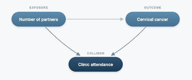
By restricting the study to clinic attendees, we’ve introduced what’s known as collider bias, which has opened up a non-causal path between the exposure and outcome. This is represented in the DAG by the two arrows pointing towards clinic attendance, making attendance a collider (a variable influenced by two other variables). While we haven’t necessarily done anything wrong with the statistical model, the bias has occurred because of how we selected the people in our study.
Mediators are also worth mentioning here because they represent another situation where adjustment can be unhelpful. Let’s consider the relationship between smoking, lung damage, and respiratory disease. In this example, lung damage is the mediator because it is one of the processes by which smoking affects respiratory health. So, if we wanted to estimate the total effect of smoking on respiratory disease, adjusting for lung damage would remove part of that effect from our analysis. Adjusting for a mediator doesn’t open a new non-causal path, but it can still be unhelpful because it removes part of the effect we’re trying to estimate.
So which variables should we adjust for?
If we consider the two examples I’ve already described, we can see that adjusting for a variable can either be helpful or introduce bias. So how do we know which variables we should adjust for?
The difference comes down to how each variable is related to the exposure and outcome, and DAGs can help us visualise this. By drawing out the assumed causal relationships, we can identify which variables we should adjust for to reduce confounding, and which ones we should avoid adjusting for because doing so could introduce bias. To do this, we look at the different paths connecting our exposure and outcome, and consider what happens if we adjust for a variable along each path.
The aim is to adjust for variables that block non-causal paths while leaving the causal paths we’re interested in open. In more complicated DAGs, there may be several combinations of variables that allow us to do this, which are known as sufficient adjustment sets. In the table below I’ve summarised the three types of variables we’ve discussed, and what we need to consider when deciding whether to adjust for them.
| Variable | What it means | Should we adjust for it? | How it appears in a DAG* |
|---|---|---|---|
| Confounder | A common cause of the exposure and outcome, like maternal age in our birth order example | Generally yes, to block non-causal paths and reduce confounding | Exposure ← Confounder → Outcome |
| Collider | An effect of two variables, like clinic attendance in the cervical cancer example | Generally no conditioning on it as it opens a non-causal path | Exposure → Collider ← Outcome |
| Mediator | A variable on the causal path between exposure and outcome, like lung damage in the smoking example | Generally no, if we’re estimating the total causal effect | Exposure → Mediator → Outcome |
* These are simplified examples. In more complicated DAGs we need to consider all the paths between the exposure and outcome before deciding which variables to adjust for.
Where do codelists come in?
Once we’ve used a DAG to decide which confounders we need to adjust for, we still have to identify those variables in our data and adjust for them. In the birth order example, maternal age is relatively straightforward to calculate if we have accurate dates of birth and delivery, however many variables used in epidemiological research are much harder to define particularly when we’re working with electronic health records (EHRs).
Imagine, for example, that our DAG identifies diabetes as an important confounder. If we’re working with EHRs, there might not be one single variable that reliably tells us which patients have diabetes. Instead, we may need to identify them using a collection of clinical codes recorded in their health records.
This is where codelists come in handy. A codelist defines which codes we use to identify a particular condition or clinical concept in health data. As such, the quality of the codelist is very important. If it is too narrow, we might miss the patients with diabetes, because their records contain codes we haven’t included. In this instance, even though we’ve correctly identified diabetes as a confounder in our DAG, we may not have captured it accurately enough to fully account for its influence on our analysis, potentially leaving us with residual confounding. Conversely, if it’s too broad, we could incorrectly identify patients with having diabetes, for example by including too many codes.
This is why identifying the right variables to adjust for is only part of the process. A DAG helps us decide what we need to measure, while good-quality codelists help us to identify the medical details in routinely collected health data.
Summary
The most important thing to take away from this post is that the relationships between variables matter just as much as the variables themselves. DAGs give us a way to think through and visualise these relationships before we start our analysis, which can help us make our assumptions explicit, as well as identify an appropriate adjustment strategy. Of course, DAGs are only as reliable as the assumptions we make when building them, and even when we’ve identified the right variables, we still need to make sure we’ve measured them accurately in our data.
If you’re interested in this topic and would like to learn more, I recommend the following:
- What is a confounder, really? - A more detailed explanation of confounders and how they differ from mediators and colliders.
- What do we mean by bias in health data research? - The different types of bias in health data, including collider bias.
- What is the difference between selection bias and sampling bias? - How the way we select people for a study can influence our findings.
- What is a codelist? - How clinical concepts are defined and identified in routinely collected health data.
- Tutorial on Directed Acyclic Graphs - Digitale, Martin and Glymour (2022), Journal of Clinical Epidemiology. A useful introduction to DAGs, causal paths and adjustment strategies.
Enjoyed this? Subscribe to my newsletter.
I write about open science, research code, and building better tools for researchers.


