How Synthetic Data Gets Made

Caroline Morton

August 9, 2026
This post is an introduction to some of the common methods used to generate synthetic data. This is intended to be a high level overview without going into a ton of detail for each methodology. Each method has (or will eventually have) its own post that goes into more detail about how it works, some of the advantages and disadvantages and its potential use cases.
Two camps of synthetic data generation
If you read a systematic review of synthetic data generation methods, you will often see the methods of synthetic data generation split into two camps: data-driven and process-driven. I think this is a useful distinction to make because it tells you how much you need access to real data, and from that we can make some inferences about the privacy and bias implications. The two camps are:
- Data Driven - requires real data to learn the structure of what data looks like and then generates new data that is similar to the real data. In my experience, this is most common and would include many machine learning approaches such as GANs, VAEs and Diffusion models.
- Process Driven - does not require real data but instead requires some domain knowledge and possibly some published statistics. You create a model of what you think the data should look like and then generate new data from that model.
Splitting the methods into these two camps is useful but there is also a hybrid approach, which I talk about later on in this blog.
Data-driven: Use the real data to drive your model
Data driven methods require access to real data in order to recreate the structure of the data. This is very much in the wheelhouse of machine learning, where the model learns the structure of the data and then generates new data that is similar to the real data. In general we are talking about row-level access to real data, rather than summary statistics. In the healthcare setting, this likely means access to patient-level row data where each row represents an event in the patient’s health history. This is the sort of data that is the most sensitive and requires the highest level of privacy protection.
The methods that fall into this category include:
Generative Adversarial Networks (GANs)
I have written a separate post that goes into a lot more detail but in short, GANs are a machine learning approach that uses two networks in competition with each other. One network (called the generator) generates new data by learning the structure of the real data. The other network (called the discriminator) tries to distinguish the real data from the generated data. Over time, the generator gets better at generating data that looks like the real data.
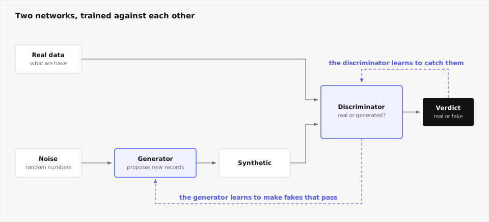
GANs were very popular in the past but have some limitations and are not quite as common now. The main risk here is mode collapse - where the generator gets very good at generating a small number of examples that are good at tricking the discriminator, rather than being representative of the real data.
Variational Autoencoders (VAEs)
VAEs are another machine learning approach that uses two networks, but instead of them being in competition, they are used together to learn a compressed representation of the data. The first network (the encoder) takes the real data and compresses it down into a compact representation, called the “latent space”. This means a simplified version of the data that captures the key underlying patterns. The second network (the decoder) takes that compressed representation and tries to reconstruct the original data from it.
The “variational” part means that the encoder doesn’t just produce a single value for each data point (like for example, a point age for a population of patients with a particular disease), but instead produces a small range of possible values. Once the model is trained, you can generate new data by sampling a random point from that latent space and passing it through the decoder alone. VAEs are generally considered more stable and easier to train than GANs but the downside is that the outputs are often less sharp since the model is optimising for a good average (a distribution). This is often described as “blurry” outputs.
There are also Conditional VAEs (CVAEs) but I will cover those within the post on VAEs themselves.
Diffusion Models
Diffusion models are the newer approach in machine learning and actually have become pretty popular in the last few years for image generation (think about that next time you see a generated image of a cat on a skateboard).

The core idea is that you take the real data and gradually add noise to it, step by step until you end up with random noise. The model then learns how to reverse this process. Once the model has learned this denoising process, you can generate new data by starting with random noise and running the model to denoise it step by step until you end up with realistic-looking data.
The downside of diffusion models is that they are made up of many many small steps so they tend to be a bit slower compared to GANs or VAEs. The upside though is that they do not suffer from the mode collapse that GANs are prone to, and they tend to produce sharper outputs (less blurry) than VAEs. They naturally produce a wide range of outputs because each one starts from a different random noise pattern.
Copulas
Copulas are a statistical approach for generating data and do not use neural networks. The approach is to split the problem into two parts: what each variable looks like on its own, and how the variables relate to each other. This first part is called the “marginal distribution” and it is just the shape of each individual variable as a distribution (like say a bell curve for age, or a skewed distribution for blood pressure or inflammatory markers). The second part is the “dependence structure” and it captures how the variables move together. For example, how age and blood pressure tend to increase together. It doesn’t worry about the individual shape of each of these variables, only how they relate to each other.
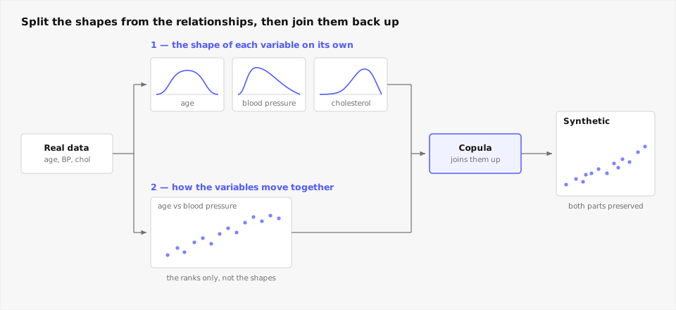
Copulas then work by combining these parts back together to generate realistic joint data. Joint data just means combined data that makes sense together. For example, a realistic age and blood pressure pairing. This isn’t limited to just two variables either - copulas can capture the dependence structure across many variables at once, so a simulated patient’s age, blood pressure, cholesterol, and BMI can all be generated together in a way that’s realistic as a whole set.
There are several advantages. Firstly they are built on a well understood statistical theory rather than the black-box of a neural network so they tend to be much more explainable as you can see why a model is generating the data it is. They also tend to be pretty fast to fit and they don’t require the enormous amounts of data that neural networks often do.
The downside is that they tend to struggle with very high-dimensional data - you can imagine the “joint” distribution of hundreds of variables is a lot more complex than just a two or three.
CART (Classification and Regression Trees)
CART is another statistical approach for generating synthetic data, and again it doesn’t rely on neural networks. This time it doesn’t model each variable once on its own but in sequence. It builds a decision tree for each variable that predicts the output of that variable based on the values of the other previous variables. So in simple terms, it is asking the question at the “blood pressure” variable: “given the age, sex, BMI and cholesterol of this patient, what is the most likely blood pressure?” and then it generates a new value by sampling from that tree. It does this for each variable in turn, building up a full synthetic record one variable at a time.
This tends to be a bit more flexible than others, like copulas, because it doesn’t care about the shape of the distribution of each variable or the relationships between them. It just wants to predict the next variable based on the previous ones. This can mean that it is good at creating more complex relationships between variables - particularly non-linear relationships or effect modification - which are common in real-world data. It is also pretty good at handling a range of variable types, like numeric, categorical and binary variables all in the same dataset. This is a significant advantage because real clinical datasets are often a mix of these types.
The downside is that because each variable is generated conditionally on the ones before it, the order you choose to generate variables in can affect the quality of the output, and errors or quirks introduced early in the sequence can propagate through to later variables.
Fitted Bayesian Networks
Bayesian networks are another statistical approach, this time using a graphical model called a directed acyclic graph (DAG). Instead of looking at the data as a table of rows and columns, you represent it as a graph where each variable is a node, and the arrows between the nodes show which variables directly influence which others. So age would have an arrow pointing to blood pressure, representing that age has an influence on blood pressure.
Fitted here means that the network has learnt from real data, both the structure of the graph itself (which nodes, and which arrows between them) and the strength of each of those relationships. The DAG is not hand-drawn in advance, it comes out of the dataset you are working with.
Once the network is fitted, you generate new synthetic records by sampling through the graph. You start with the variables that have no arrows pointing into them, generate values for those, then move on to the variables that depend on them, using the values you have just generated to inform the next ones, and carry on until every variable in the record has been filled in.
The advantage is that it can capture complex relationships, and I think it is much easier to understand conceptually when you can see the graph. The downside is that with a lot of variables the graph gets very complex and hard to learn correctly, and if the graph is wrong then so are the relationships baked into the model. Most implementations also assume fairly simple relationships by default, often linear ones, which we know is often not the case in real world data.
Large Language Model (LLM) based
This is a new one for me but I have added this in here because I think this is going to be more and more important. By this point we are all familiar with LLMs and their ability to create text from data that it has trained on. The idea here is that you take each row of your dataset and instead of treating it like a dictionary of variables (like age: 45, sex: female, blood_pressure: 120), you serialise it into a string of text. You then take a pre-trained LLM and fine-tune it on your dataset. The model learns the structure of the data in the same way that it learns how sentences and paragraphs are structured in natural language. Once the model is trained, you can generate new rows of data by prompting it to create a new “sentence” that looks like the rows it has seen before.
Multiple imputation and perturbation
I include this here although as I state in my post on multiple imputation and perturbation, these are not really methods of synthetic data generation. They are statistical techniques that are sometimes repurposed for synthetic data generation, but they are not well suited to the task. Multiple imputation is designed to fill in missing data, and perturbation is designed to add noise to real data.
What all these data-driven methods have in common
There are some commonalities between all of these data-driven methods, most obviously that they require access to real data in order to learn the structure of the data. This is usually, if not always, row level data that is the most identifying and sensitive. I have written about privacy in synthetic data in a separate post here and privacy vs utility here.

What is good about these methods is that they take advantage of the computational power now available to surface structure that we would not have found on our own. Our brains can only hold so much information to pattern match on, but a neural network can learn from millions of rows at once. This can make the synthetic data it generates more representative of the real data, and really this is the major selling point of the approach.
The downside is that bias in the data is inherited by the model (and often amplified - you can read my blog on bias amplification for more on this). Small subsets of the data that are underrepresented in the real data are often underrepresented in the synthetic data or lost altogether. This has downstream consequences not only for rare diseases but patients who are rare in several different dimensions (e.g. an unusually young patient with a fairly rare disease, from an underrepresented ethnic group). The model has seen very few examples of this type of patient and therefore it is unlikely to generate many examples of them in the synthetic data.
The other major downside is the black box nature of some of these methods, particularly the machine learning approaches. They generate good synthetic data often but it is less explainable and I worry that it is possible that real data could be memorised by the model and therefore disclosed in the synthetic data. This poses a risk of privacy that is hard to quantify and even harder to mitigate.
Process-driven: describe how the world works, then run a model based on these descriptions
Process driven methods are a completely different approach. They do not require access to row level data - but they do require some domain knowledge and possibly some published statistics. The basic idea is that you create a model of how the world works and then you run a model based on that to generate some synthetic data. This is a totally different approach to the data-driven methods.
The sorts of methods that fall into this category include:
Rules-based

This is the simplest approach and the easiest to understand. You write down the rules that govern the relationships between variables and then generate the data that follows those rules. For example, you could write down that a patient’s age must be between 18 and 80 years old, and that a patient’s blood pressure must be between 90 and 180 mmHg. You also write down that a patient’s blood pressure increased by X mmHg for every 10 years of age. You then generate a dataset that follows these rules. This is a very simple example but you can see how this could be extended to more complex rules and relationships between variables. You can of course add in randomness to the rules (perhaps the blood pressure increases by 1 to 5 mmHg for every 10 years of age) to make the data more realistic. It all sounds quite simple but you actually get quite a lot of mileage out of this approach, because luckily we know quite a lot about how the human body works and how diseases progress. You can write down a lot of rules and relationships between variables and they are often enough to generate a realistic dataset that is useful for testing pipelines and doing analysis.
Disease state graphs
This approach models a disease as a set of discrete health states - for example, Healthy, Mild Disease, Moderate Disease, Severe Disease, and Deceased - connected by arrows that represent the probability of moving from one state to another over time. This is often governed by what’s called a Markov chain, where the probability of moving to the next state depends only on the state you are currently in and not on how you got there. Once the graph is built, you generate synthetic patients by “walking” them through it over simulated time steps, so that what you end up with is a longitudinal disease history for each patient rather than a single snapshot at one point in time.
The advantages are that it is a very visual approach, so you can see the states and understand the transitions between them, and that the probabilities are explicit and can be traced back to their source if you have done it correctly.
The requirement is that you need good published estimates to build those transition probabilities in the first place - incidence rates, age-specific mortality tables, illness duration distributions - and the synthetic histories you generate are only ever as good as those estimates. Where the estimates do not exist you end up filling the gaps with expert opinion, which is hard to do well and brings its own selection bias, since a respiratory consultant and a GP will give you different answers about the same patient.
Agent-based / microsimulation
This method takes the disease state graph idea a step further and combines elements of rule based as well. Instead of modelling a single condition as a set of states, you model each patient as an independent “agent” with their own set of characteristics - age, sex, comorbidities, behaviours - and simulate how those characteristics evolve and interact over time, according to a set of rules you define. Each agent moves through simulated time on its own, making its own transitions, so you end up with a population of independently simulated patients rather than just a single disease trajectory.

The scope tends to be much bigger than a disease state graph. The agent can track many different things about the patient at once. You can also allow agents to interact with each other, which makes it particularly useful for modelling infectious disease spread, where whether one agent becomes infected depends on which other agents they come into contact with. It also has some interesting applications at the population level when thinking about behaviours of groups (like uptake of vaccines or screening programmes) and how an individual’s behaviour is not completely self-determined but influenced by the behaviour of others in their social network.
The downsides are that it is more complex and computationally expensive to run at scale and can be hard to validate its correctness. I think this is one of the most interesting parts of synthetic data generation and I can see there being really interesting applications of this in the future, far beyond infectious disease modelling. It is a very flexible approach and the computational power at our fingertips now means that in theory we can simulate very large populations of patients.
Discrete event simulation
This is a more traditional operational research approach that is often used to model the flow of patients through a healthcare system rather than the progression of disease in individual patients. The idea is to model the system as a series of discrete events - a patient arriving at a clinic, being seen by a doctor, having tests done, receiving treatment, and being discharged - with each event having its own rules and probabilities attached to it.
This approach differs from the others above in an important way, because it is not really about modelling the patient’s biology but the system that the patient moves through. You are less concerned with how a disease progresses and more concerned with queues, capacity and timing, so each simulated patient is stepped through the sequence of events with waiting times and outcomes drawn from probability distributions at each stage. Run enough of them through and you end up with a synthetic dataset that reflects the operational dynamics of the system.
This makes discrete event simulation especially useful for operational and service-planning questions rather than clinical ones. The downside is much the same as the other process-driven methods here: you need a good understanding of the real system and its underlying probability distributions to build an accurate model. I know from experience that hospitals are vastly different from place to place, and even within a single hospital the pathways can be different.
Schema-driven / faker-style
Schema driven is a very simple approach that is often overlooked. It is the idea of generating data based on a schema or template - for example like a schema of a patient discharge summary or the schema of a clinical trial dataset or the schema of the event table from a data provider like CPRD. You source the structure of the data from the schema and then generate random values for each field based on the type of data it is. For example, if a field is a date, you generate a random date within a certain range. If a field is a categorical variable, you randomly select one of the categories, and so on. You can also add in some simple rules to make the data more realistic - for example, you can’t die from a disease before you are born.
In my opinion this is a seriously underrated approach for testing pipelines - particularly data ingestion pipelines where you want to make sure that your code can handle a variety of inputs, edge cases and missing data. If you just want to make sure that your code will execute when presented with unexpected missing values or negative values in a blood pressure, you don’t need to worry about the data being realistic.
What all these process-driven methods have in common
These approaches are all mediated on one thing: your own understanding of your problem space and what you can encode into a model. This means that you are not learning things from the data model itself but it is forcing you to think about and write down your knowledge about that data model. All of these techniques are constrained by what you put in meaning that if you don’t know about a relationship between two variables, it won’t be in the model and therefore it won’t be in the synthetic data. This is a very different approach to the data-driven methods. The upside of this is that you can audit the model by reading it rather than having to do an analysis on the output and compare it to the real data. You can see exactly what relationships are being modelled.
With all of these methods, there is a much reduced risk of disclosure because you are not using any real data to generate the synthetic data. The only caveat here is how are you sourcing that knowledge? If you are using published statistics, then you are probably fine. If you are using the real data to get summary statistics, then you are edging back into the data-driven camp and you need to be careful about disclosure risk.
Finally, there are of course biases in the assumptions you make and the knowledge you encode into the model. This is a different type of bias to the data-driven methods, but it is still bias.
Side by side
Here is a side-by-side comparison of the two approaches. This is not exhaustive but it is a good starting point to understand the differences between the two approaches.
| Data-driven | Process-driven | |
|---|---|---|
| What you need | row-level real records | domain knowledge, published statistics |
| Structure comes from | the data | you |
| Can surface structure you did not know about | yes | no |
| Disclosure risk | by construction | none, if no individual data was used |
| Where the bias comes from | the source data, invisibly | your assumptions, explicitly |
| Scales with | number of variables | your patience! |
| Breaks when | data is small, or the subgroup is rare | the system is too complex to write down |
| Audit by | measuring the output | reading the model |
It is a spectrum, not a binary
Finally I want to mention something I referred to in the introduction: this is not a binary choice between data-driven and process-driven. Increasingly I see what I would call hybrid approaches that combine elements of both approaches. This might be as simple as looking at the real dataset to get your summary statistics and then using those to inform a process-driven model, or it might be more complex like using a data-driven model to generate synthetic data and then applying a rules-based layer on top to fix any impossible records. There are many different ways to combine the two approaches and in my opinion, this is where a lot of the interesting work is happening and is going to happen in the future. We are more rich in data than ever before but we are so much more aware of the privacy risks now than in the past. There is a strong desire to walk that line between privacy and utility and I think hybrid approaches can really go a long way to achieving that balance.
Conclusion
There is no best method in this list. The first question to ask is what is the use case of the synthetic data? What is the minimal requirement for the synthetic data to be useful for that use case? What is the acceptable level of risk in terms of bias and disclosure? The answers to these questions will guide you to the right method for your use case.
The thing I want to hammer home is that there is no perfect option here (there is no free lunch as the saying goes). Every method has its own strengths and weaknesses, and bias gets in no matter what you do, but it looks a little different with each method. The only way to guard against all the weaknesses and potential biases is to write down what you did, particularly preserving the code that generated the synthetic data, and to be transparent about the limitations of the synthetic data you are using. This is particularly important if you are sharing or publishing the synthetic data for others to use.
Further reading
For more information on synthetic data, you might find the following resources useful:
- Synthetic Data Series - series page with links to all the posts in the series, including this one.
- What is Synthetic Data?
- Synthetic Data Use Cases in Healthcare Research
Enjoyed this? Subscribe to my newsletter.
I write about open science, research code, and building better tools for researchers.